This panel provides for the entry of draw curve data and its visualization, for the calculation of bow energy by means of its draw curve.
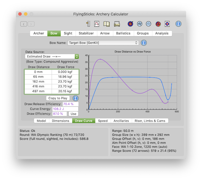
As a bow is progressively drawn, the force required at different draws is plotted. The area under this curve is a measure of the energy transferred from the archer's mussels to the bow. A large proportion of this energy is subsequently transferred to the arrow as kinetic energy. Note the draw curve is based on static measurements as distance and force measurements are taken.
When an arrow is released, it is accelerated by a force from the bow. The plot of this force versus distance traveled is the release curve. It might be expected that this would be the inverse of the draw curve - however that is never the case due to dynamic effects. The release is fast, so inertia of the arrow and various bow parts come into play. (A static release curve may be measured and it will be similar to the draw curve - but will show some hysteresis).
Select a source of draw curve data to display in the Data Table below. There are six options:
Estimated from Bow ParametersPresents limited set of estimated values based on the current bow type and its parameters, particularly draw weight and draw length. While the data may not be edited, the units of measurement may be changed in the usual way. The add and remove row buttons are hidden. For non-compound bow, just 5 data pairs are used to describe the draw curve due to the simplicity of the curve. For compound bows, 9 data pairs are required due to the drop-off and valley characteristics. These are minimalist data sets. Measured Draw CurveFor bow draw data that has been physically measured. Allows up to 20 data pairs to be entered and edited. If you have collected more than 20 measurement pairs, then do not use the ones where the curve is relatively straight. Note that the draw distance is measured from the brace position where the draw force is assumed zero. All fields can be edited except for the first row. This data set is saved with the bow parameters. Play SetA draw curve data set for your experimentation. Data can be copied into this are using the Copy to Play Set button. Can be edited as for the Measured Draw Curve data. The Play Set data set is saved with the bow parameters. Release Curve EstimateShows the main data points for the estimated release curve. Influenced by many bow and arrow parameters. The draw curve used is the last selected draw curve (i.e. measured, estimated or play set). Note the release curve force is the force applied to accelerate the arrow. It takes into account the energy loss due to the bow's virtual mass. Measured Release CurveGathering this data is hard! Use high speed photography, arrow instrumented with an accelerometer, optical sensor with striped arrow, etc. With present FlyingSticks, only measures energy imparted to arrow, however as the simulation model is developed, various tuning parameters may become available. Full Draw LengthBy default shows a vertical line at the full draw distance (i.e. draw length minus brace height). Addition vertical lines may be added. The fields are editable, but the draw force is always shown as "#####". |
The draw curve plot associated with the selected Data Source is highlighted in bright blue, the related curve in light blue with the others left in place for comparison but in a subdued grey.
Immediately below the Data Source selection is a reminder of the bow type that is assumed in calculating the estimates. This is as selected on the Bow>Model panel.
The data table shows the draw distance from brace (or power stroke) in the left column and the draw force in the right column. The table is always sorted in ascending order by draw distance, no matter what order the data in entered.
The measurement units may be changed in the usual way and all entries in the column and the adjacent plots will reflect that change.
If the add row button is visible, then clicking it will add a new row after the last row and will have its two fields set to "#####" indicating they are waiting for data entry. Once the distance field is entered the row is likely to be moved by the automatic sorting process.
If the remove row button is visible, then clicking it will remove the currently selected row. The removal is final and can not be undone. If no row is selected, no action is taken.
If visible, clicking will copy the selected draw curve data to the Play Set from where it can be manipulated and experimented with. The original Play Set data will be lost.
Show the ratio of the release curve energy to the draw curve energy for the last selected draw curve. These are the energies represented by the area under the respective curves. Note the release curve energy becomes the arrow's kinetic energy. This is not to be confused with the available energy that is available to accelerate both the arrow AND the bow's virtual mass.
If the selected data source is a draw curve, this is the calculated potential energy transferred to the bow by the archer in drawing the bow. If the selected data source is the release curve, then it is the energy transferred to the arrow. In both cases, it is effectively the area under the curve.
If the data does not extend to the archers full draw length, the field is shown in red, indicating the value will be in error. The obvious solution is to extend the data to or beyond the draw length.
This is the ratio of the arrow PLUS bow virtual mass kinetic energy (as per the speed selected in Bow>Speed) to the currently selected draw or release curve. For draw curves this is typically 75% to 85%. If it is outside this range there is probably something wrong with the draw curve, the speed source or the arrow mass specification.
For the estimated release curve the efficiency should be close to 100% if the estimate is reasonable. However the parametric model is not perfect, so some deviation can be expected.
Transfers the draw curve Draw Efficiency to to the bow's nominal Draw Efficiency.
Draw curves from the available sources are displayed here with automatic scaling. The data points are shown with point marks (e.g. +, x, o) and a smooth line is draw passing through each point.
The smoothing algorithm assumes the data points belong to a smooth system, so if a point is too far from the expected, the whole curve can look very strange. (The curve fitting is not by a least square regression as might have been expected, but instead a Bezier spline fit). Where finer detail is required (such as in the valley region of a compound bow), the data points should be closer together to assist the fitting process.
The curve corresponding to the selected Data Source is highlighted in bright blue for easy identification. If present the light blue trace is that data related to the selected data - thus if the Estimated Draw curve is selected then the light blue trace will be the Estimated Release Curve. And, visa versa if the Estimated Release is then selected.
Cycling through the Data Sources allows identification of the various curves.
Provides the usual access to this page within a popup window.
As mentioned above, the release curve is an estimate. Presently FlyingSticks takes a parametric approach in defining features on the curve. Each feature's form, position and amplitude is a function of various bow and arrow parameters. This is most certainly a compromise compared to the potentially more rigorous and traditional finite element approach. However apart from the extra computing power required, the finite element method requires vastly more detail about the bow's properties - well beyond what most archers would be able to measure or quantify.
Several observations can be made. Compound bows behave very differently to non-compounds due to the relatively high mass of the pulleys at the end of the limbs. This mass absorbs energy early after release but returns it towards the end of the power stroke as can be seen with the kick in the release curve. Reflex bows can exhibit a similar but much smaller effect.
A well designed or evolved war bow will ensure the string tension nearing brace height is increased significantly by the forces required to decelerated the limbs towards the end of the launch cycle. This kinetic energy of the limb is significant and is obviously best transferred to the arrow rather than the destruction of the bow. The shape, mass distribution and strength distribution of the limbs all contribute in this regard.
Any system containing springs and masses tends to oscillate. With a system as complicated as the bow and arrow, there are many superimposed oscillation modes. The FlyingSticks parametric model only attempts to model the fundamental longitudinal oscillation.
Conclusion - regard the release curve as no more than an indicative aid in understanding the complexities of the bow's internal ballistics. Hopefully in future a more advanced model with realistic inputs will be developed.